|
|
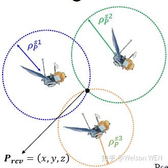
Global navigation satellite system (GNSS)是无人车定位中的关键一个部分. GNSS是当前唯一一个可以提供绝对定位信息的一种信息来源.无人车的基于地图匹配定位的这一个部分中,GNSS经常用来提供初始化.就目前来看,GNSS的定位方式主要包括单点定位(SPP),也就是我们手机常用的定位方式;RTK定位和DGNSS定位. 本次介绍单点定位的原理,求解及其代码实现。假设有三颗卫星,每颗卫星的位置知道,每颗卫星距离接收机的距离(pseudorange)也是知道,即可以通过:
(1) WLS方法计算接收机的位置
x^*=(G^T G)^{-1}G^T\rho \tag{1}
\boldsymbol{G}=\left[\begin{array}{cccc} {\frac{\left(x^{1}-x_{i}\right)}{\rho_{i}^{1}}} & {\frac{\left(y^{1}-y_{i}\right)}{\rho_{i}^{1}}} & {\frac{\left(z^{1}-z_{i}\right)}{\rho_{i}^{1}}} & {1} \\ {\frac{\left(x^{2}-x_{i}\right)}{\rho_{i}^{2}}} & {\frac{\left(y^{2}-y_{i}\right)}{\rho_{i}^{2}}} & {\frac{\left(z^{2}-z_{i}\right)}{\rho_{i}^{2}}} & {1} \\ {\frac{\left(x^{3}-x_{i}\right)}{\rho_{i}^{3}}} & {\frac{\left(y^{3}-y_{i}\right)}{\rho_{i}^{3}}} & {\frac{\left(z^{4}-z_{i}\right)}{\rho_{i}^{3}}} & {1} \\ {\frac{\left(x^{4}-x_{i}\right)}{\rho_{i}^{4}}} & {\frac{\left(y^{4}-y_{i}\right)}{\rho_{i}^{4}}} & {\frac{\left(z^{4}-z_{i}\right)}{\rho_{i}^{4}}} & {1} \end{array}\right] (2)
其中 (x_i, y_i, z_i) 为接收机位置,
其中 (x^{i},y^{i}, z^{i}) 为第i颗卫星的位置;
\rho ^ { ( k ) } ( t ) = r ^ { ( k ) } ( t , t - \tau ) + \underbrace { c \left[ \partial _ { u } ( t ) - \delta t ^ { ( k ) } ( t - \tau ) \right] } _ { \text { Clock Enors } } + I ^ { ( k ) } ( t ) + T ^ { ( k ) } ( t ) + \varepsilon _ { \rho } ^ { ( k ) } ( t ) \tag{3}
The matrix G is the line vector from receiver to satellite. \rho is the pseudorange measurement. x^* is the position estimate of the GNSS receiver. For more detail, refer to reference.
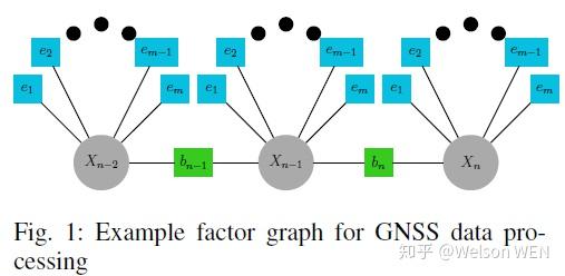
(2) 基于图优化的GNSS单点定位(framework of principle)
With the development and popular usage of graph optimization in SLAM probelm, the graph optimization begins to be used in GNSS SPP. Some research related to this method.
{ e _ { i } = H _ { i } \left( X _ { i } \right) - Z _ { i } }\tag{4}
{ \hat { X } = \operatorname { argmin } \sum \left\| e _ { i } \right\| _ { \Sigma } ^ { 2 } }\tag{5}
\left\| e _ { p r } ^ { j } \right\| _ { \Sigma _ { j } } ^ { 2 } = \left\| \rho _ { I F } ^ { j } - \hat { \rho } _ { I F } ^ { j } \right\| _ { \Sigma _ { j } } ^ { 2 } = e _ { p r } ^ { j } \Sigma _ { j } ^ { - 1 } e _ { p r } ^ { j } \tag{6}
If the switchable constraints are available, then we can obtain improved cost/optimization function as:
\begin{aligned} \hat { X } , \hat { S } = \underset { X , S } { \operatorname { argmin } } & \sum _ { i } \left\| e _ { p r } ^ { i } \right\| _ { \Sigma } ^ { 2 } \\ & + \sum _ { i } \left\| \psi \left( s _ { i } \right) * e _ { p r } ^ { i } \right\| _ { \Sigma } ^ { 2 } \\ & + \sum _ { i } \left\| \gamma _ { i } - s _ { i } \right\| _ { \Xi } ^ { 2 } \end{aligned}\tag{7}
- Team from Tsinghua University:
A Robust Graph Optimization Realization of Tightly Coupled GNSS-INS integrated navigation system for urban vehicles
- Team from WVU:
- Evaluation of kinematic precise point positioning convergence with an incremental graph optimizer
- Robust Navigation In GNSS Degraded Environment Using Graph Optimization
- Team from TU Chemnitz
- Reisdorf, P., Pfeifer, T., Breßler, J., Bauer, S., Weissig, P., Lange, S., Wanielik, G. & Protzel, P. (2016) The Problem of Comparable GNSS Results — An Approach for a Uniform Dataset with Low-Cost and Reference Data. In Proc. of Intl. Conf. on Advances in Vehicular Systems (VEHICULAR). ISBN: 978-1-61208-515-9
- Pfeifer, T., Weissig, P., Lange, S. & Protzel, P. (2016) Robust Factor Graph Optimization — A Comparison for Sensor Fusion Applications. In Proc. of Intl. Conf. on Emerging Technologies and Factory Automation (ETFA)
- Sünderhauf, N., Obst, M., Lange, S., Wanielik, G. & Protzel, P. (2013) Switchable Constraints and Incremental Smoothing for Online Mitigation of Non-Line-of-Sight and Multipath Effects. In Proc. of IEEE Intelligent Vehicles Symposium (IV). DOI: 10.1109/IVS.2013.6629480
- Sünderhauf, N., Obst, M., Wanielik, G. & Protzel, P. (2012) Multipath Mitigation in GNSS-Based Localization using Robust Optimization. In Proc. of IEEE Intelligent Vehicles Symposium (IV). DOI: 10.1109/IVS.2012.6232299
- Sünderhauf, N. & Protzel, P. (2012) Towards Robust Graphical Models for GNSS-Based Localization in Urban Environments. In Proc. of IEEE International Multi-Conference on Systems, Signals and Devices (SSD). DOI: 10.1109/SSD.2012.6198059
- Sünderhauf, N. (2012) Robust Optimization for Simultaneous Localization and Mapping. PhD: Chemnitz University of Technology
(3) 基于紧耦合的EKF定位
TODO: EKF-based tight coupling of GNSS. Adaptive Estimation of Measurement Noise to Improve the Performance of GNSS Single Point Positioning in Dense Urban Environment.
Actually, we can employ the EKF to tightly estimate the receiver's position with observation of pseudorange. Results shown from papers [5] shows that improved results are obtained using adaptive error covariance tunning. This implementation can be find in RTKLIB.
基于系统状态方程的非线性,扩展卡尔曼滤波提出线性化过程如下:
大部分的状态估计问题都包含非线性方程:
x_t=g(u_t, x_{t-1})
z_t=h(x_t)
其中个 g(x) 和 h(x) 均包含非线性成分。
Prediction的线性化:
g(u_t,x_{t-1})\approx g(u_t,\mu_{t-1})+\frac{\partial g(u_t,\mu_{t-1})}{\partial x_{t-1}}(x_{t-1}-\mu_{t-1})
g(u_t,x_{t-1})\approx g(u_t,\mu_{t-1})+G_t(x_{t-1}-\mu_{t-1})
Correction的线性化:
h(x_t)\approx h(\bar{\mu_t})+\frac{\partial h(\bar{\mu_t})}{\partial x_{t}}(x_t-\bar{\mu_t})
h(x_t)\approx h(\bar{\mu_t})+H_t(x_t-\bar{\mu_t})
扩展卡尔曼滤波公式(具体公式推导待更新)
Prediction:
(EKF) \bar{\mu_t}=g(u_t,\mu_{t-1})\Leftarrow (KF:) \bar{\mu_t}=A_t\mu_{t-1}+B\mu_{t}
(EKF) \bar{\Sigma_t}=G_t\Sigma_{t-1}G_{t}^{T}+Q_{t} \Leftarrow (KF) \bar{\Sigma_t}=A_t\Sigma_{t-1}A_{t}^{T}+Q_{t}
Correction:
(EKF) K_t=\bar{\Sigma_t}H_{t}^{T}(H_t\bar{\Sigma_t}H_{t}^{T}+R_t)^{-1} \Leftarrow (KF): K_t=\bar{\Sigma_t}C_{t}^{T}(C_t\bar{\Sigma_t}C_{t}^{T}+R_t) ^{-1}
(EKF): \mu_t=\bar{\mu_t}+K_t(Z_t-h_t\bar{\mu_t}) \Leftarrow (KF): \mu_t=\bar{\mu_t}+K_t(Z_t-C_t\bar{\mu_t})
(EKF) \Sigma_t=(I-K_t H_t)\bar{\Sigma_t} \Leftarrow (KF): \Sigma_t=(I-K_tC_t)\bar{\Sigma_t}
(\mu_t,\Sigma_t)
通过对比EKF和KF的公式会发现,主要区别在于
A_t\Leftrightarrow G_t
C_t\Leftrightarrow H_t
对于计算雅克比矩阵,假设状态向量为 X_t=[x_i,y_i,v_{x,i},v_{y,i}]^{T} ,观测向量为 z_t=[R_i,\theta_i]^{b} 。根据 z_t=h(x_t) 。
\left[ \begin{matrix} R_i \\ \theta_i \end{matrix} \right] = \left[ \begin{matrix} h_1(x_1) \\ h_2(x_2) \end{matrix} \right] \tag{8}
h_1 (x_t)=\sqrt{(x_i^{2}+y_i^{2})} \tag{9}
h_2 (x_t)=arctan(\frac{y_i}{x_i}) \tag{10}
H_t (2\times4)= \left[ \begin{matrix} \partial h_1(x_t)/\partial x_i & \partial h_1(x_t)/\partial y_i & \partial h_1(x_t)/\partial v_{x,i} & \partial h_1(x_t)/\partial v_{y,i} \\ \partial h_2(x_t)/\partial x_i & \partial h_2(x_t)/\partial y_i & \partial h_2(x_t)/\partial v_{x,i} & \partial h_2(x_t)/\partial v_{y,i} \\ \end{matrix} \right] \tag{11}
对于 H_t 矩阵的大小:m*n (m为观测向量的维度,n为状态向量的维度)。
Update:
For EKF-based GNSS SPP, the measurement update of a state vector x and its covariance matrix P are represented by a measurement vector z_k at epoch k as
\widehat { x } _ { k } = \widehat { x } _ { \overline { k } } + K _ { k } \left( z _ { k } - h \left( \widehat { x } _ { \overline { k } } \right) \right)\tag{12}
P _ { k } = \left( I - K _ { k } H \left( \widehat { x } _ { \overline { k } } \right) \right) P _ { \overline { k } }\tag{13}
\boldsymbol { K } _ { k } = \boldsymbol { P } _ { \overline { k } } \boldsymbol { H } \left( \hat { x } _ { \overline { k } } \right) ^ { T } \left( \boldsymbol { H } \left( \hat { \boldsymbol { x } } _ { \overline { k } } \right) \boldsymbol { P } _ { \overline { k } } \boldsymbol { H } \left( \hat { \boldsymbol { x } } _ { \overline { k } } \right) ^ { T } + \boldsymbol { R } _ { k } \right) ^ { - 1 } \tag{14}
where \hat{x}_k and P_k are the state vector and its covariance matrix before the measurement update. h(x) is the measuremnet model vector. H(x) is the matrix of partial derivatives (Jac matrix). R is the measurement noise covariance.
Predict:
Assuming the system model is linear, the time update of the state vector and its covariance matrix are expressed by
\begin{aligned} \hat { \boldsymbol { x } } _ { \overline { k } } & = \boldsymbol { F } _ { k } \hat { \boldsymbol { x } } _ { k - 1 } + \boldsymbol { D } _ { k } \boldsymbol { u } _ { k } \\ \boldsymbol { P } _ { \overline { k } } & = \boldsymbol { F } _ { k } \boldsymbol { P } _ { k - 1 } \boldsymbol { F } _ { k - 1 } ^ { T } + \boldsymbol { Q } _ { k } \end{aligned} \tag{13~14}
Reference:tnd Q_k are the transition matrix and the covariance matrix of the system noise from epoch k-1 to k . Importantly, D_k relates relates the optional control input u_k to the state vector.
State and observation matrix calculation:
GNSS SPP defines the measurement equations as follows:
\rho^{i}=\gamma^{i}+\sigma t+\varepsilon_{\rho_{i}}\tag{15}
where \rho^{i} is the pseudo-range in meters from satellite i . Note that there are satellite clock errors, ionospheric errors and tropospheric errors, one need to estimates this first. \sigma t is the receiver clock bias. \varepsilon_{\rho_{i}} is the measurement noise caused by for example, NLOS/Multipath!
The unknown state vector can be defined as
\begin{array} { c } { x_t = \left( \boldsymbol { g } _ { u } , \delta t , \dot { \boldsymbol { g } } _ { u } \right) ^ { T } } \\ { \boldsymbol { g } _ { u } = \left( x _ { u } , y _ { u } , z _ { u } \right) } \\ { \dot { \boldsymbol { g } } _ { u } = \left( \dot { x } _ { u } , \dot { y } _ { u } , \dot { z } _ { u } \right) } \end{array} \tag{16}
Be noted that:
- { g } _ { u } = ( x _ { u } , y _ { u } , z _ { u } ) denotes the user position in ECEF in an earth-centered (ECEF) coordinate frame. P in PVT
- { \dot { \boldsymbol { g } } _ { u } =( \dot { x } _ { u } , \dot { y } _ { u } , \dot { z } _ { u } ) } denotes the velocity of user in meters. V in PVT
- \delta t denotes the receiver clock bias in meters. T in PVT
z = ( \boldsymbol { \rho } ) ^ { T }\tag{17}
\boldsymbol { \rho } = \left( \rho ^ { 1 } , \rho ^ { 2 } , \cdots , \rho ^ { m } \right)\tag{18}
\boldsymbol { h } ( \widehat { \boldsymbol { x } } ) = ( \gamma ) ^ { T }=z\tag{19}
\gamma = \left( \gamma ^ { 1 } + \delta t , \gamma ^ { 2 } + \delta t , \cdots , \gamma ^ { m } + \delta t \right) \tag{20}
\gamma ^ { i } = \left\| g ^ { i } - g _ { u } \right\|\tag{21}
\boldsymbol { g } ^ { i } = \left( x ^ { i } , y ^ { i } , z ^ { i } \right)\tag{22}
\boldsymbol { a } _ { u } ^ { i } = \frac { g ^ { i } - \boldsymbol { g } _ { u } } { \left\| \boldsymbol { g } ^ { i } - \boldsymbol { g } _ { u } \right\| }\tag{23}
where g^{i} is the position of i_{th} satellite. Assuming that we have 6 satellites.
z=\left[ \begin{matrix} z_1 \\ z_2 \\ z_3 \\ z_4 \\ z_5 \\ z_6 \end{matrix} \right]=\left[ \begin{matrix} \gamma ^ { 1 } + \delta t \\ \gamma ^ { 2 } + \delta t \\ \gamma ^ { 3 } + \delta t \\ \gamma ^ { 4} + \delta t \\ \gamma ^ { 5 } + \delta t \\ \gamma ^ { 6} + \delta t \end{matrix} \right]=\left[ \begin{matrix} h_1(x) \\ h_2(x) \\ h_3(x) \\ h_4(x) \\ h_5(x) \\ h_6(x) \end{matrix} \right]\tag{24}
h_i(x)=\sqrt{( (x^{i}-x_u)^{2} + (y^{i}-y_u)^{2} + (z^{i}-z_u)^{2})}\tag{25}+\delta_{t}
x_t=\left[ \begin{matrix} x_u \\ y_u \\ z_u \\ \delta_t \\ v_x \\ v_y \\ v_z \end{matrix} \right] \tag{26}
Ja matrix的大小为6*7,因此矩阵 H_t 为
H_t=\frac{\partial h(\bar{\mu_t})}{\partial x_{t}} \tag{27}
H_t=\left[ \begin{matrix} \frac{\partial h_1(x_t)}{\partial x_{u}} & \frac{\partial h_1(x_t)}{\partial y_{u}} & \frac{\partial h_1(x_t)}{\partial z_{u}} & \frac{\partial h_1(x_t)}{\partial \delta_{t}} & \frac{\partial h_1(x_t)}{\partial v_{x}} & \frac{\partial h_1(x_t)}{\partial v_{y}} & \frac{\partial h_1(x_t)}{\partial v_{z}} \\ \frac{\partial h_2(x_t)}{\partial x_{u}} & \frac{\partial h_2(x_t)}{\partial y_{u}} & \frac{\partial h_2(x_t)}{\partial z_{u}} & \frac{\partial h_2(x_t)}{\partial \delta_{t}} & \frac{\partial h_2(x_t)}{\partial v_{x}} & \frac{\partial h_2(x_t)}{\partial v_{y}} & \frac{\partial h_2(x_t)}{\partial v_{z}}\\ \frac{\partial h_3(x_t)}{\partial x_{u}} & \frac{\partial h_3(x_t)}{\partial y_{u}} & \frac{\partial h_3(x_t)}{\partial z_{u}} & \frac{\partial h_3(x_t)}{\partial \delta_{t}} & \frac{\partial h_3(x_t)}{\partial v_{x}} & \frac{\partial h_3(x_t)}{\partial v_{y}} & \frac{\partial h_3(x_t)}{\partial v_{z}} \\ \frac{\partial h_4(x_t)}{\partial x_{u}} & \frac{\partial h_4(x_t)}{\partial y_{u}} & \frac{\partial h_4(x_t)}{\partial z_{u}} & \frac{\partial h_4(x_t)}{\partial \delta_{t}} & \frac{\partial h_4(x_t)}{\partial v_{x}} & \frac{\partial h_4(x_t)}{\partial v_{y}} & \frac{\partial h_4(x_t)}{\partial v_{z}} \\ \frac{\partial h_5(x_t)}{\partial x_{u}} & \frac{\partial h_5(x_t)}{\partial y_{u}} & \frac{\partial h_5(x_t)}{\partial z_{u}} & \frac{\partial h_5(x_t)}{\partial \delta_{t}} & \frac{\partial h_5(x_t)}{\partial v_{x}} & \frac{\partial h_5(x_t)}{\partial v_{y}} & \frac{\partial h_5(x_t)}{\partial v_{z}} \\ \frac{\partial h_6(x_t)}{\partial x_{u}} & \frac{\partial h_6(x_t)}{\partial y_{u}} & \frac{\partial h_6(x_t)}{\partial z_{u}} & \frac{\partial h_6(x_t)}{\partial \delta_{t}} & \frac{\partial h_6(x_t)}{\partial v_{x}} & \frac{\partial h_6(x_t)}{\partial v_{y}} & \frac{\partial h_6(x_t)}{\partial v_{z}}\end{matrix} \right]\tag{28}
For matrix R:
\boldsymbol { R } = \left( \begin{array} { c c } { \boldsymbol { R } _ { \rho } } & { } \\ { } & { \boldsymbol { R } _ { \dot { \boldsymbol { \rho } } } } \end{array} \right)\tag{29}
R _ { \rho } = \operatorname { diag } \left( \sigma _ { \rho ^ { 1 } } ^ { 2 } , \sigma _ { \rho ^ { 2 } } , \ldots , \sigma _ { \rho ^ { m } } ^ { 2 } \right)\tag{30}
\sigma _ { p n } = 2 , \sigma _ { p n } = 1 \\ P _ { 0 } = \operatorname { diag } \left( 10 ^ { 2 } , 10 ^ { 2 } , 10 ^ { 2 } , 10 ^ { 2 } , 1 ^ { 2 } , 1 ^ { 2 } , 1 ^ { 2 } , 1 ^ { 2 } \right)\tag{31}
\sigma _ { \rho } ( S N R ) = 0.64 + 784 * e ^ { - 0.142 * S N R }\tag{32}
For Prediction or time update:
\begin{aligned} \boldsymbol { F } & = \boldsymbol { I } , \boldsymbol { D } _ { k } = \boldsymbol { I } \cdot \Delta t _ { k } \\ \boldsymbol { u } _ { k } & = \left( \dot { x } _ { u , k - 1 } , \dot { y } _ { u , k - 1 } , \dot { z } _ { u , k - 1 } , \dot { \delta } t _ { k - 1 } , 0,0,0,0 \right) ^ { T } \end{aligned}\\ Q = \left( \begin{array} { c c c } { \boldsymbol { Q } _ { g _ { u } } } & { } & { } \\ { } & { \sigma _ { p \delta t } ^ { 2 } } \\ { } & { } & { \boldsymbol { Q } _ { \hat { g } _ { u } } } \\ { } & { } \end{array} \right) \\ \begin{aligned} Q _ { g _ { u } } & = \operatorname { diag } \left( \sigma _ { p x } ^ { 2 } , \sigma _ { p y } ^ { 2 } , \sigma _ { p z } ^ { 2 } \right) \\ \boldsymbol { Q } _ { \dot { g } _ { u } } & = \operatorname { diag } \left( \sigma _ { p x } ^ { 2 } , \sigma _ { p \dot { y } } ^ { 2 } , \sigma _ { p \dot { z } } ^ { 2 } \right) \end{aligned}\tag{33}
TODO: Adaptive estimation of the covariance matrix in [5]
Reference:
- Groves, Paul D.Principles of GNSS, inertial, and multisensor integrated navigation systems. Artech house, 2013.
- Li, Wei, Xiaowei Cui, and Mingquan Lu. "A robust graph optimization realization of tightly coupled GNSS/INS integrated navigation system for urban vehicles."Tsinghua Science and Technology23.6 (2018): 724-732.
- Evaluation of kinematic precise point positioning convergence with an incremental graph optimizer
- Robust Navigation In GNSS Degraded Environment Using Graph Optimization
- Adaptive Estimation of Measurement Noise to Improve the Performance of GNSS Single Point Positioning in Dense Urban Environment.
- https://ags.cs.uni-kl.de/fileadmin/inf_ags/opt-ss12/lec10_opt.pdf
香港理工大学定位于导航实验室近期招聘研究助理(需有研究生学位),博士生,博士后。研究方向包括GNSS RTK定位,多传感融合定位(因子图优化,factor graph optimization)。有意联系微信:welsonpolyu |
|


 发表于 2022-11-5 12:00:37